Calculate transfer functions • proxysnr

Overview

This vignette explains, for the two special cases of isotope diffusion in polar firn and time uncertainty in layer-counted chronologies, how to calculate spectral transfer functions which describe the expected loss in spectral power as a function of frequency. For time uncertainty, the loss applies to the spectrum of the common signal recorded by the spatial average of an array of layer-counted proxy records (the “stacked” record); for diffusion, it applies to the loss in average spectral power of individual isotope records.

The documentation utilises as examples the code for calculating the transfer functions for the DML and WAIS isotope records studied in Münch and Laepple (2018). There, you will also find a detailed description of the basic method (see Appendix B).

Dependencies

library(proxysnr)

For the modelling of time uncertainty the suggested package simproxyage is required, so we need to check whether it is available:

has.simproxyage <- proxysnr:::check.simproxyage()
#> 
#> Checking simproxyage availability... ok.

In case you have not installed simproxyage and you try to rebuild this vignette, you will receive a message with installation instructions here. The vignette will still build, though without actually calculating any time uncertainty transfer function.

General settings

First, we set up general variables and parameters that are required for the calculations.

For convenience, list objects are used for saving the transfer functions:

# for diffusion transfer function
dtf <- list()
# for time uncertainty transfer function
ttf <- list()

A specific resolution of the created surrogate white noise time series is used for the diffusion calculations, for which, in general, a higher resolution compared to the target resolution of the isotope records is adopted. This is necessary for numerical stability of the diffusion results at the high-frequency end.

Here, the target resolution of the isotope records is 1 yr (annual resolution) and a simulation resolution of 0.5 yr has proven sufficient for the numerical stability of the results:

res <- 1/2

Finally, we specify the number of Monte Carlo simulations used to obtain the transfer functions. In general, an average of a large number of simulations is needed to reduce the spectral uncertainties and obtain smooth estimates. However, to reduce computation time, only a small number of simulations is used here for the vignette:

ns <- 10

Note that for the results of Münch and Laepple (2018), ns has been set to 100,000, which required a computation time of 1–3 hours depending on the dataset (using a 2.4 GHz Intel Core i5 processor).

DML1 isotope records

In the following, we document all dataset-specific parameters needed for the calculations along the example of the DML1 dataset of isotope records.

Specify the number of proxy records (“cores”) in the studied array:

nc <- 15

Specify the time axis common to all proxy records in the array in units of the original (target) resolution of the records (here, years), which gives the number of proxy data points:

# set time axis
t <- seq(1994, 1801)
# number of proxy data points
nt <- length(t)

Specify the time points of age control points where the time uncertainty is assumed to be zero:

acp <- c(1994, 1884, 1816, 1810)

Set the rate of the random process which perturbs the proxy record chronologies, so here the rate of missing or double-counting of a layer; we use symmetric rates here:

rate <- 0.013

(Specify a numeric vector with two entries to use asymmetric rates.)

For the diffusion simulations, estimates of the diffusion length (in units of the record resolution) are needed as a function of time since deposition. Along with proxysnr, the diffusion length estimates for the DML and WAIS cores are provided in the internal dataset diffusion.length. Calculation of these estimates is documented in the package source under ./data-raw/produce-internal-data.R, where . is the root of the package source directory. For further information see the publication Münch and Laepple (2018).

We can now run the diffusion model,

set.seed(4122018)
dtf$dml1 <- CalculateDiffusionTF(nt = nt / res, nc = nc, ns = ns,
                                 sigma = proxysnr:::diffusion.length$dml1[, -1],
                                 res = res)

and the time uncertainty model with Gaussian white noise as surrogate data:

set.seed(4122018)
if (has.simproxyage) {
  suppressMessages(
    ttf$dml1 <- CalculateTimeUncertaintyTF(t = t, acp = acp, nt = nt, nc = nc,
                                           ns = ns, rate = rate,
                                           surrogate.fun = rnorm)
  )
} else {
  ttf <- NULL
}

The other isotope records

We run the calculations for the DML2 isotope records…

set.seed(4122018)

nc <- 3
t <- seq(1994, 1000)
nt <- length(t)
acp <- c(1994, 1884, 1816, 1810, 1459, 1259)
rate <- 0.013

dtf$dml2 <- CalculateDiffusionTF(nt = nt / res, nc = nc, ns = ns,
                                 sigma = proxysnr:::diffusion.length$dml2[, -1],
                                 res = res)

if (has.simproxyage) {
  suppressMessages(
    ttf$dml2 <- CalculateTimeUncertaintyTF(t = t, acp = acp, nt = nt, nc = nc,
                                           ns = ns, rate = rate,
                                           surrogate.fun = rnorm)
  )
}

… and the WAIS isotope records:

set.seed(4122018)

nc <- 5
t <- seq(2000, 1800)
nt <- length(t)
acp <- c(2000, 1992, 1964, 1885, 1837, 1816, 1810)
rate <- 0.027

dtf$wais <- CalculateDiffusionTF(nt = nt / res, nc = nc, ns = ns,
                                 sigma = proxysnr:::diffusion.length$wais[, -1],
                                 res = res)

if (has.simproxyage) {
  suppressMessages(
    ttf$wais <- CalculateTimeUncertaintyTF(t = t, acp = acp, nt = nt, nc = nc,
                                           ns = ns, rate = rate,
                                           surrogate.fun = rnorm)
  )
}

Plot the transfer functions

The obtained transfer functions can be plotted with:

PlotTF(dtf = dtf, ttf = ttf,
       names = c("DML1", "DML2", "WAIS"),
       col = c("black", "firebrick", "dodgerblue"))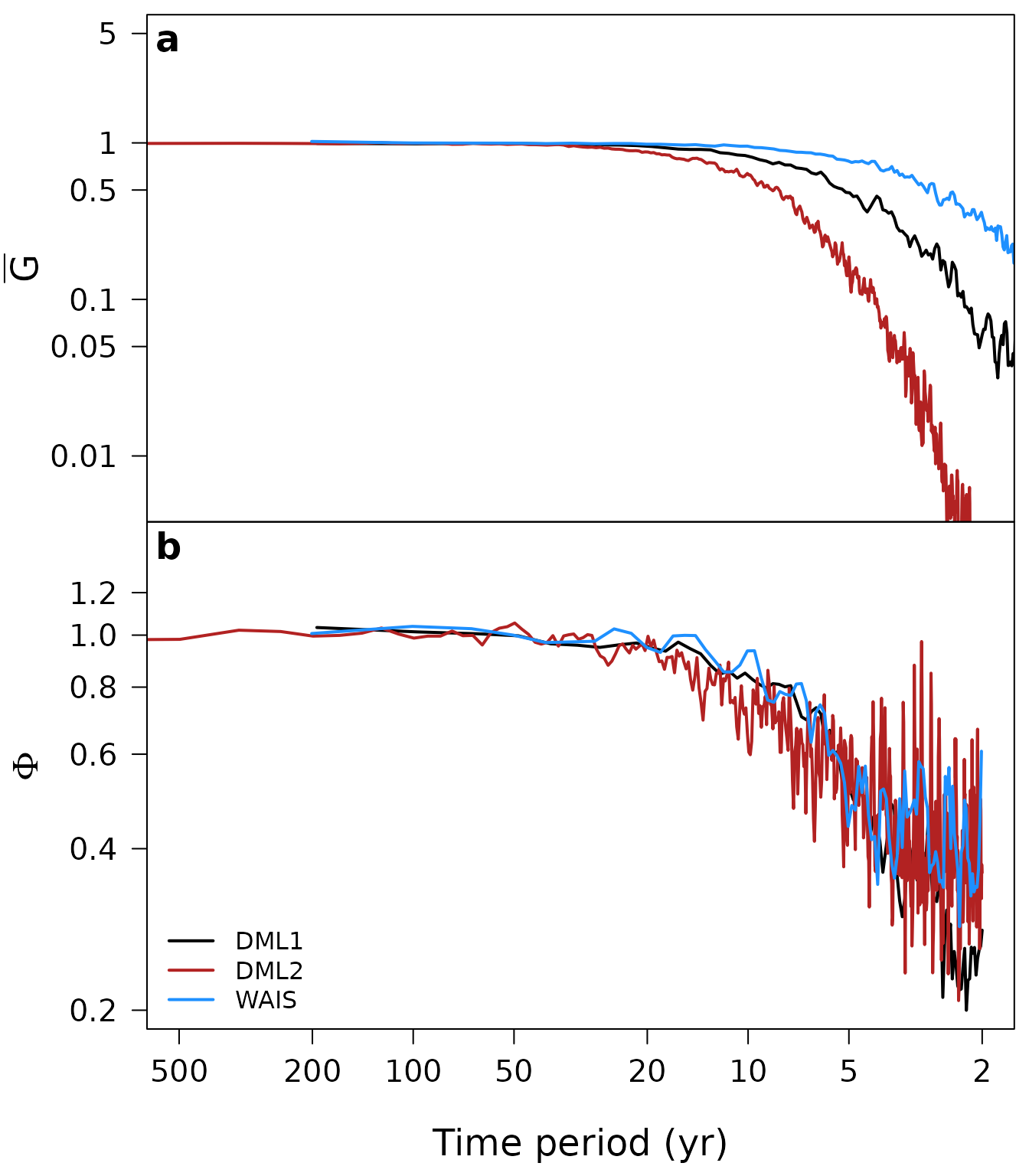

Fig. 1: Estimates of the spectral transfer functions for the effects of site-specific diffusion (a) and time uncertainty (b) for three arrays of firn-core isotope records: DML1 (black), DML2 (red) and WAIS (blue) (as studied in Münch and Laepple, 2018). Plotted is in each case the average transfer function from 10 Monte Carlo simulations.

The transfer functions for simulations with ns = 10^5 as used and shown in Münch and Laepple (2018), Fig. B1, are provided along proxysnr in the variables ?diffusion.tf and ?time.uncertainty.tf.

These can be plotted by simply omitting the transfer function parameters in the plot call:

PlotTF(names = c("DML1", "DML2", "WAIS"), dtf.threshold = 0.5,
       col = c("black", "firebrick", "dodgerblue"))

Literature cited

Münch, T. and Laepple, T.: What climate signal is contained in decadal- to centennial-scale isotope variations from Antarctic ice cores?, Clim. Past, 14, 2053-2070, doi: 10.5194/cp-14-2053-2018, 2018.