The following objects are masked from 'package:stats':

    filter, lag
The following objects are masked from 'package:base':

    intersect, setdiff, setequal, union
library(tidyr)
5.1 Errors on the power spectrum of single timeseries
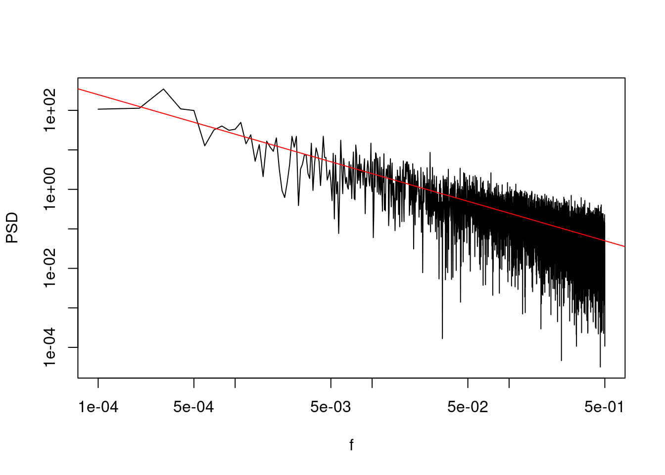
If the power spectrum of a stochastic timeseries is estimated using the basic Fourier transform method, i.e. we take the raw periodogram with no smoothing, padding or tapering, then the power spectral density estimates are exponentially distributed around their expected value (true value if we know it). They are equivalently described as “chi-squared” distributed with 2 degrees of freedom, or “gamma” distributed with shape = 1, scale = 1. The exponential is a special case of the gamma, and the gamma will be useful later on.
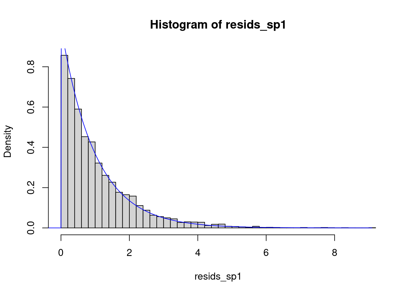
Here we demonstrate this by simulating a timeseries, using R’s function for getting the periodogram, calculating the residuals from the “true” spectrum, creating a histrogram of the residuals, and overlaying the probability density function for the exponential distribution.
We define the “residuals” as the ratio of the estimated PSD \(\hat{S}\) to the true PSD \(S\).
\[ \frac{\hat{S}}{S} \]
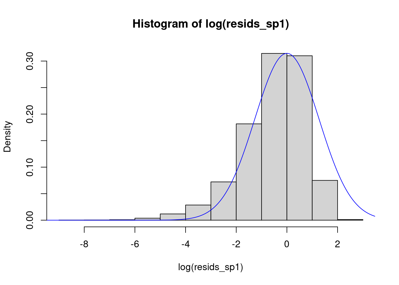
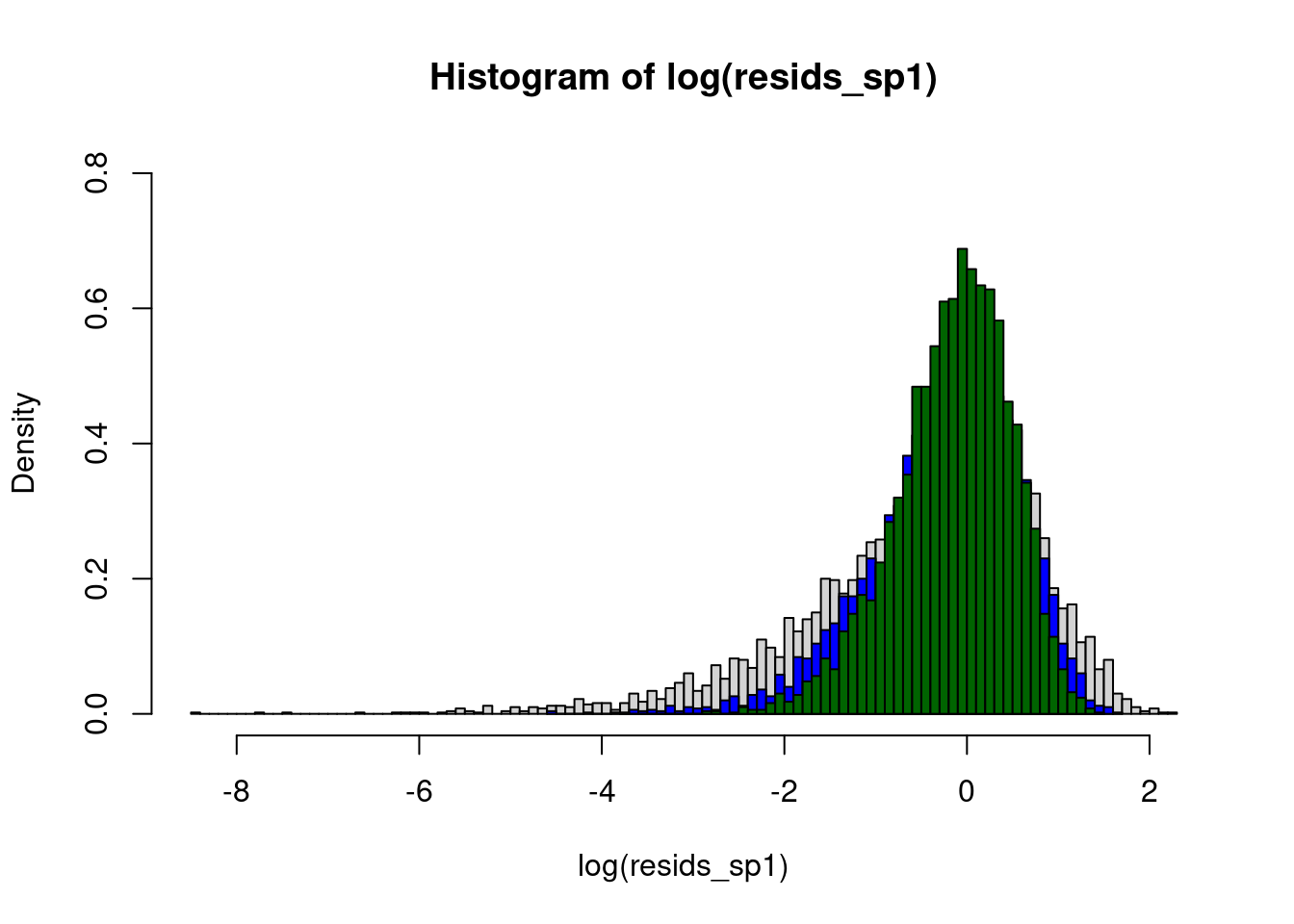
Or equivalently the difference in the log of these values
\[
\log{\hat{S}} - \log{S}
\]
n <-1e04alpha <-0.025beta =1t1 <-sim.proxy.series(nt = n, a = alpha, b = beta)sp1 <-spec.pgram(t1, taper =0, plot =FALSE)LPlot(sp1)abline(a =log10(alpha), b =-beta, col ="red")
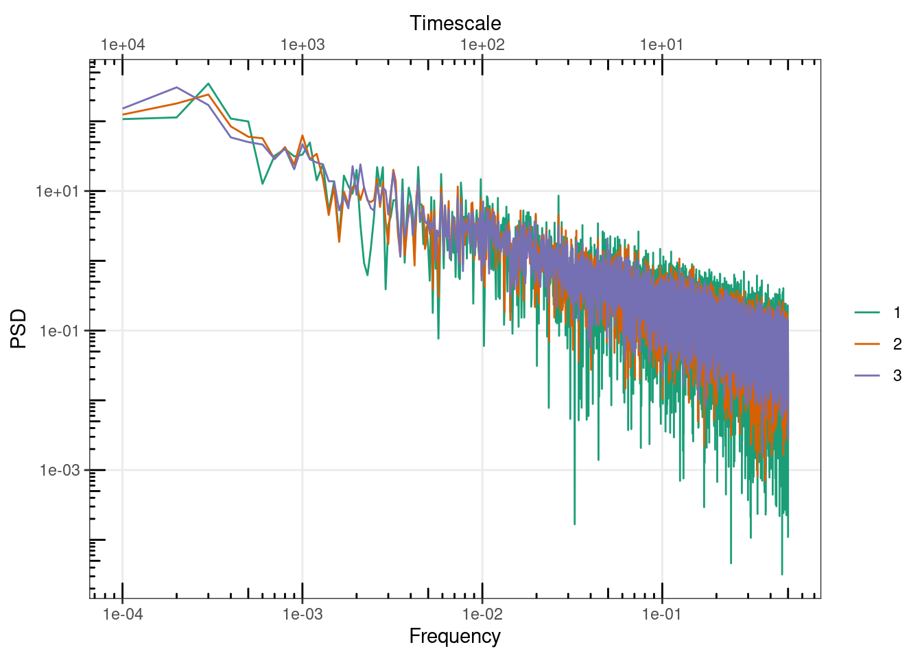
5.2 Errors on the mean spectrum of multiple timeseries
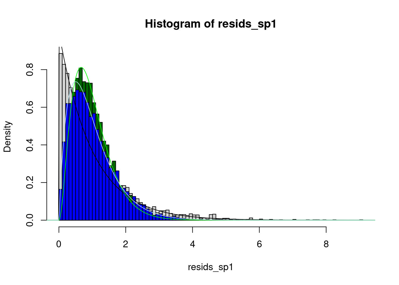
With a single time series the errors are exponentially distributed, a special case of the gamma distribution with shape = 1 and scale = 1. More generally, if we estimate the power spectra of multiple, n, timeseries and then calculate the mean power spectrum, the errors of this mean spectrum are gamma distributed with shape = n and scale = 1/n (or shape = n, rate = n).
This follows as the gamma distribution is the “sampling distribution” of the exponential. That is, if you take means of samples of size n from an exponential distribution, the distribution of these means is gamma distributed.
t2 <-sim.proxy.series(nt = n, a = alpha, b = beta)t3 <-sim.proxy.series(nt = n, a = alpha, b = beta)t10 <-replicate(10, {sim.proxy.series(nt = n, a = alpha, b = beta)})# The SpecACF function can take a matrix of timeseries and return the mean spectrumsp2 <-SpecACF(cbind(t1, t2), 1)sp3 <-SpecACF(cbind(t1, t2, t3), 1)sp10 <-SpecACF(t10, 1)resids_sp2 <- sp2$spec / true_specresids_sp3 <- sp3$spec / true_specresids_sp10 <- sp10$spec / true_spec
gg_spec(list(
  sp1, sp2, sp3)
  )
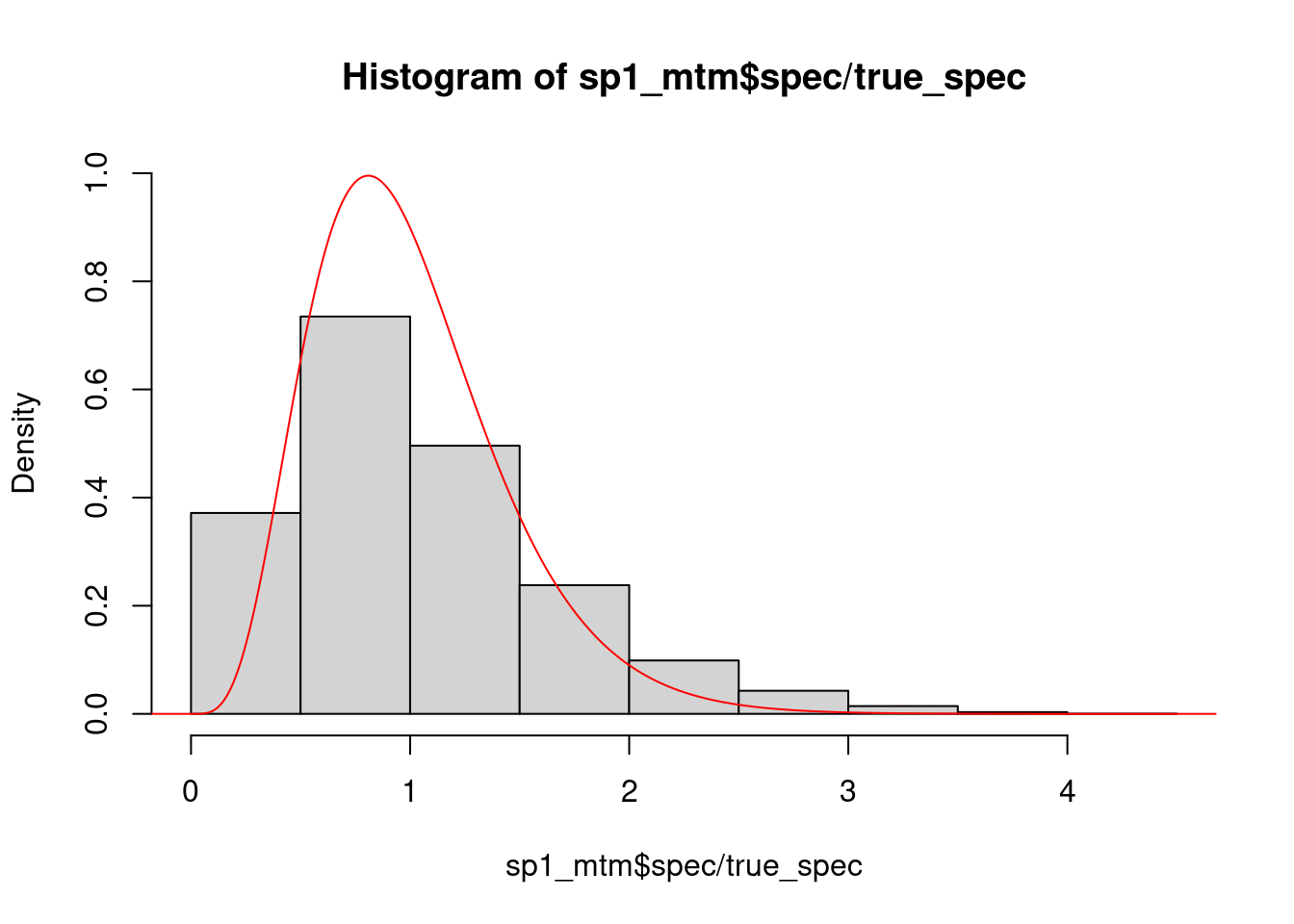
xax <-seq(-1, 20, length.out =1000)hist(resids_sp1, 100, freq =FALSE)hist(resids_sp3, 50, freq =FALSE, add = T, col ="darkgreen")hist(resids_sp2, 50, freq =FALSE, add = T, col ="blue")#hist(resids_sp10, 30, freq = FALSE, add = T, col = "red")k <-1lines(xax, dgamma(xax, k, k), col ="black")k <-3lines(xax, dgamma(xax, shape = k, scale =1/k), col ="green")k <-2lines(xax, dgamma(xax, shape = k, scale =1/k), col ="lightblue")
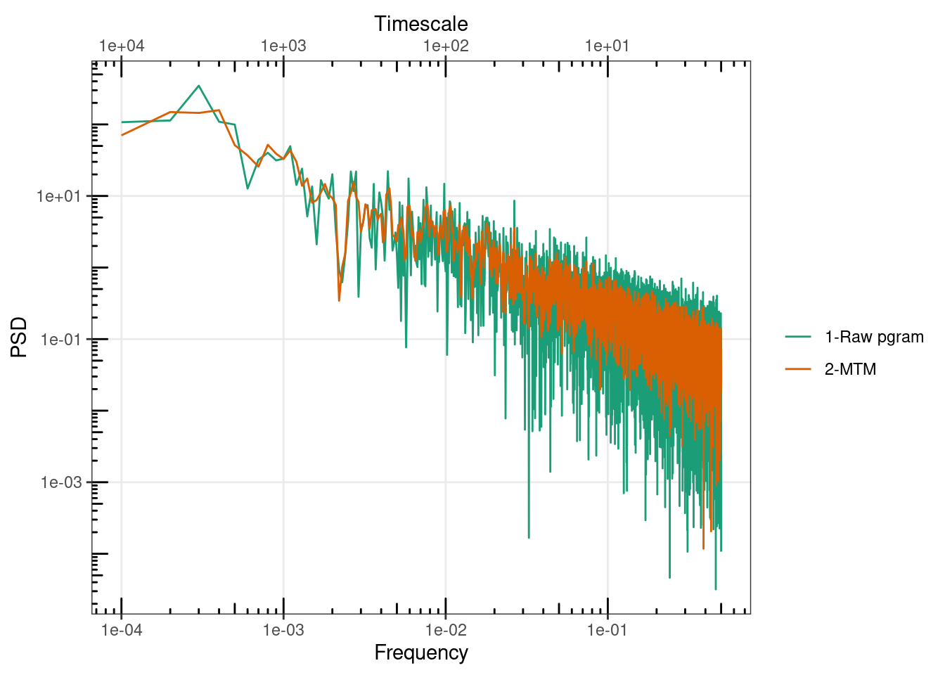
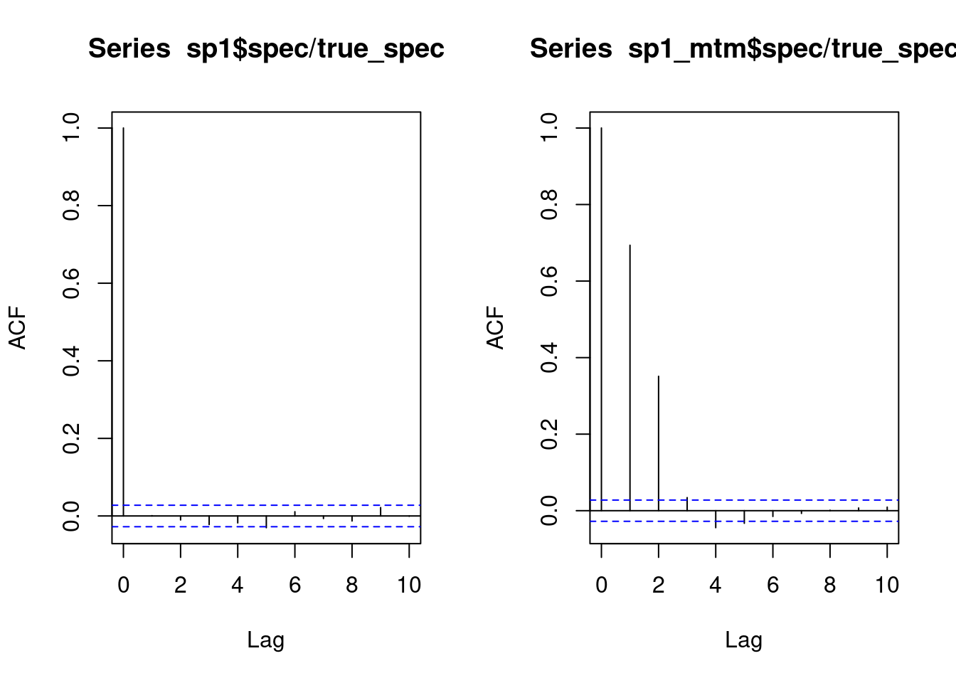
Spectral estimates using the raw periodogram, with no padding or tapering are fully independent (uncorrelated with each other) and have 2n degrees of freedom (are gamma distributed with shape = dof/2). If more sophisticated methods are used to estimate the spectrum, or if we smooth the spectrum, then this no longer holds true.
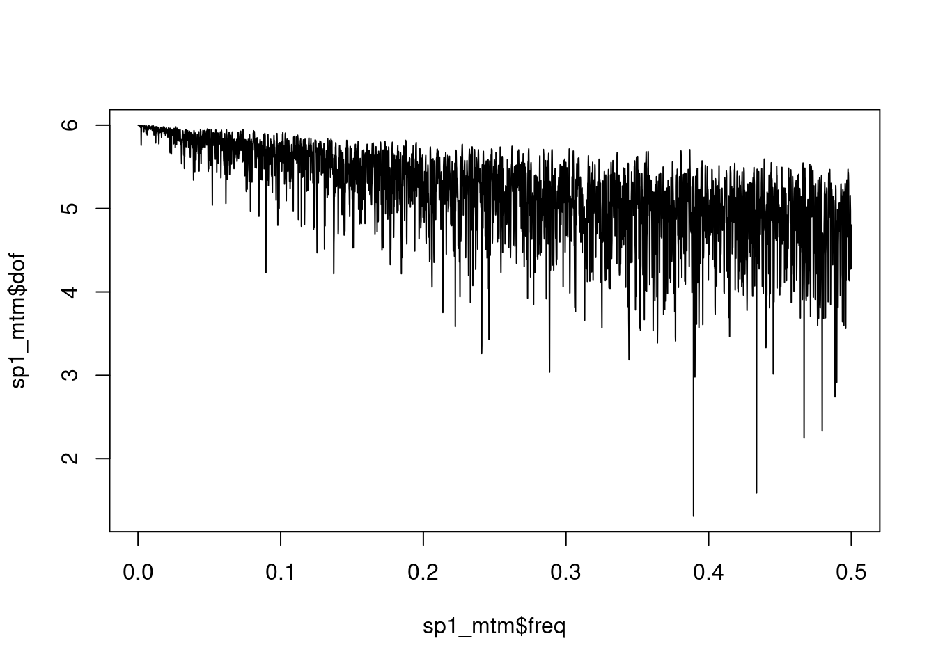
For the MTM method with the default 3 tapers, the degrees of freedom are not the same for all frequencies, and on average decline slightly with frequency.
plot(sp1_mtm$freq, sp1_mtm$dof, type ="l")
mean_dof <-mean(sp1_mtm$dof)mean_dof
[1] 5.238128
The distribution of the errors is still approximately gamma with shape equal to the mean degrees of freedom, but the errors are now serially correlated with each other.